An Introductory Look at Covariance and the Mean Vector

Introduction

When you first encounter the world of multivariate Gaussian distributions, it’s easy to feel like you’ve entered a labyrinth of equations, variables, and matrices. But beneath the mathematical machinery lies a beautifully structured framework that helps us understand complex data, and in many ways, it’s as elegant as it is powerful.

In statistics, the Gaussian, or “normal” distribution, is often our first stop when we dive into data analysis. We’ve all seen its familiar bell-shaped curve, neatly centered around a mean, showing us the most probable values a single variable might take. But in reality, data rarely exists in a vacuum. Many variables are interconnected, forming a “multivariate” data landscape where each variable influences and interacts with others. Here, the multivariate Gaussian distribution steps in as a natural extension of the single-variable Gaussian, providing us a way to model these multidimensional relationships.

At the heart of this distribution are two key players: the mean vector and the covariance matrix. The mean vector is the multivariate equivalent of the single-variable mean, summarizing the central tendencies of all variables in one go. It tells us where the “center” of our data cloud lies, capturing the average or typical values across all dimensions.

Updated on June 22, 2024: Additionally, a new blog post has been published that expands on this topic with content covering correlation coefficients and the correlation coefficient matrix.

The covariance matrix, on the other hand, is a bit like a backstage operator. It describes how variables interact with each other, revealing not just their individual spreads but also how they move in tandem. Each entry in this matrix provides insights into the relationship between pairs of variables, showing whether they rise and fall together or behave independently. Together, the mean vector and covariance matrix form a powerful duo, shaping the geometry of the distribution and giving us a complete picture of how our data points are scattered and related.

In this post, we’ll explore the roles of the mean vector and covariance matrix within the multivariate Gaussian distribution, diving into how they help us grasp and model complex data structures.

The Mean Vector – Definition and Properties

Now that we’ve opened the door to the multivariate Gaussian, let’s take a closer look at one of its core components: the mean vector. You can think of the mean vector as the “centroid” or the “anchor” point of the distribution—a snapshot of where the average of each variable in a dataset tends to lie. In a multivariate world, we don’t just care about one mean; we want to know the average value in each dimension, and that’s where the mean vector steps in.

Definition

For a multivariate random variable \(X\) with \(n\) dimensions, the mean vector \(\mu\) is defined as:

where each \(\mu_i = E[X_i]\) represents the expected value of the \(i\)-th variable. Essentially, the mean vector \(\mu\) gives us a one-stop summary of the “average” position of all dimensions, capturing the expected value along each axis of the multidimensional data space.

Derivation: Expectation of the Mean Vector

To fully appreciate the mean vector, let’s delve into its calculation using the expectation operator. Suppose \(X = \begin{bmatrix} X_1 \\ X_2 \\ \vdots \\ X_n \end{bmatrix}\) is our multivariate random variable, where each \(X_i\) is a random variable in itself. The mean vector \(\mu\) is simply the expected value of \(X\):

Breaking this down, the expectation of \(X\) is computed component-wise. That is,

This form allows us to treat each dimension independently when calculating the mean, even though they may be interdependent in terms of their distributions.

Properties of the Mean Vector

The mean vector isn’t just a passive summary of averages; it’s highly responsive to transformations, particularly linear ones. Let’s explore one of its key properties: how it behaves under a linear transformation. Consider a linear transformation where we define a new random vector \(Y\) based on \(X\) as:

where \(A\) is a constant matrix of dimensions \(m \times n\) and \(b\) is a constant vector of dimension \(m \times 1\). This setup is common in multivariate analysis, where we often transform data to new coordinate systems or scales. Here, we want to understand how this transformation impacts the mean vector.

To derive the expected value of \(Y\), we use the linearity of expectation:

Since \(A\) and \(b\) are constants, we can simplify:

So, the transformed mean vector of \(Y\) is given by \(A\mu + b\). This tells us that linear transformations shift and stretch the mean vector in predictable ways: multiplying by \(A\) scales or rotates \(\mu\), while adding \(b\) translates it. Let’s formalize this with a quick proof. Suppose \(X\) is a multivariate random variable with mean vector \(\mu = E[X]\), and we define \(Y = AX + b\). By the definition of expectation, we have:

Since \(b\) is constant, \(E[b] = b\). Additionally, because expectation is a linear operator, we get \(E[AX] = A E[X] = A \mu\). Thus,

This property is not only elegant but incredibly useful. It implies that, regardless of the transformation (as long as it’s linear), we can predict how the mean vector shifts without recalculating everything from scratch. This “transformation invariance” simplifies a lot of practical work in data analysis, letting us predict and manipulate mean vectors in transformed spaces.

In sum, the mean vector \(\mu\) isn’t just a set of averages. It’s a fundamental descriptor that tells us where our data is centered, and its behavior under transformations is both consistent and computationally friendly. Whether you’re scaling, rotating, or translating your data, the mean vector adjusts accordingly, maintaining its role as the central anchor of your multivariate Gaussian distribution.

Demo

To understand how the mean vector \(\mu\) behaves, particularly under transformations, let’s start by generating some multivariate data. We’ll create a simple 2D Gaussian distribution, calculate its mean vector, and then apply a linear transformation to see how \(\mu\) changes in response.

Here’s a Python script that does exactly this:

import numpy as np
import matplotlib.pyplot as plt

# Set a random seed for reproducibility
np.random.seed(42)

# Step 1: Define the original mean vector and covariance matrix
mu = np.array([2, 3])
cov = np.array([[1, 0.8], [0.8, 1]])  # Positive correlation between X1 and X2

# Generate a sample of 500 points from the 2D Gaussian distribution
data = np.random.multivariate_normal(mu, cov, 500)

# Plot the original distribution
plt.figure(figsize=(10, 5))
plt.scatter(data[:, 0], data[:, 1], alpha=0.5, label='Original Data')
plt.scatter(mu[0], mu[1], color='red', label='Mean Vector (Original)')
plt.xlabel('X1')
plt.ylabel('X2')
plt.title('Original Multivariate Gaussian Distribution')
plt.legend()
plt.show()

In this code, we initialize a mean vector \(\mu = [2, 3]\) and a covariance matrix with a positive correlation between the two variables. We then generate 500 points to visually represent the data cloud centered around \(\mu\).

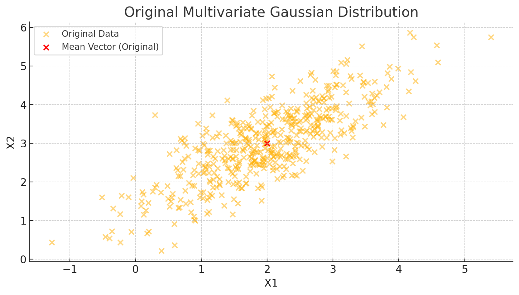
Now, let’s apply a linear transformation to this data. For demonstration, we’ll use a transformation matrix \(A = \begin{bmatrix} 1.5 & 0 \\ 0.5 & 1 \end{bmatrix}\) and a translation vector \(b = \begin{bmatrix} -1 \\ 2 \end{bmatrix}\). According to our derivation, we expect the mean vector to change to \(A\mu + b\).

# Step 2: Define the transformation matrix A and translation vector b
A = np.array([[1.5, 0], [0.5, 1]])
b = np.array([-1, 2])

# Apply the transformation to each data point
transformed_data = data @ A.T + b

# Calculate the transformed mean vector
transformed_mu = A @ mu + b

# Plot the transformed distribution
plt.figure(figsize=(10, 5))
plt.scatter(transformed_data[:, 0], transformed_data[:, 1], alpha=0.5, label='Transformed Data')
plt.scatter(transformed_mu[0], transformed_mu[1], color='blue', label='Mean Vector (Transformed)')
plt.xlabel('Y1')
plt.ylabel('Y2')
plt.title('Transformed Multivariate Gaussian Distribution')
plt.legend()
plt.show()

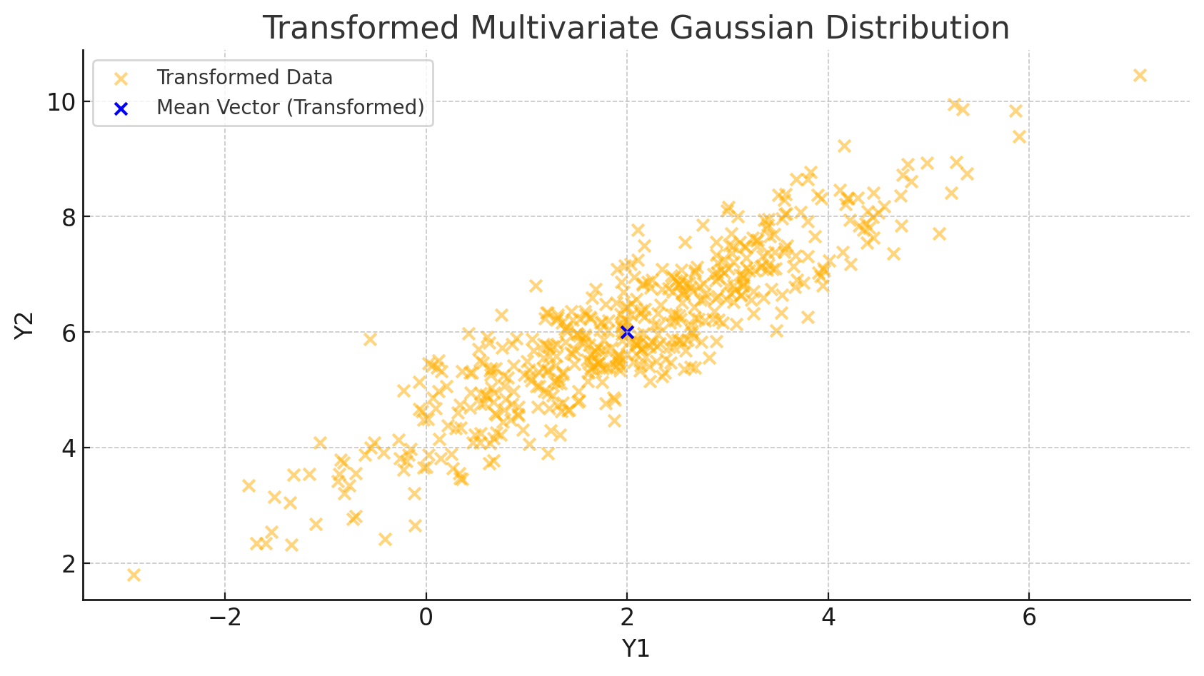
This second snippet applies our transformation and then calculates the new mean vector using \(A\mu + b\), aligning with our theoretical result. Here’s what we observe from the plot:

1. Data Shift and Rotation: The data cloud shifts according to the translation vector \(b\) and stretches based on the transformation matrix \(A\).
2. Mean Vector Update: The new mean vector \(\mu\) moves precisely to \(A\mu + b\), as predicted.

Covariance Matrix – Definition and Computation

If the mean vector \(\mu\) gives us a sense of location, then the covariance matrix \(\Sigma\) gives us a sense of shape. It describes how variables are spread and how they relate to each other, capturing both individual variances and pairwise covariances.

Definition

The covariance matrix \(\Sigma\) of a multivariate random variable \(X = \begin{bmatrix} X_1 \\ X_2 \\ \vdots \\ X_n \end{bmatrix}\) is defined as:

where each element \(\Sigma\_{ij} = \text{Cov}(X_i, X_j)\) is the covariance between \(X_i\) and \(X_j\).

Covariance, in essence, measures the degree to which two variables vary together. When \(i = j\), \(\Sigma\_{ii} = \text{Var}(X_i)\), representing the variance of \(X_i\) itself.

Derivation: The Formula for Covariance

To formally compute \(\Sigma\), let’s start with the mean vector \(\mu\) of \(X\), defined as:

Now, the covariance matrix is calculated as the expectation of the outer product of the deviations of \(X\) from its mean:

This formula may look abstract, but it’s grounded in a straightforward concept: by centering \(X\) around its mean (i.e., subtracting \(\mu\)) and then taking the outer product, we capture the spread and co-spread of each variable pair.

Step-by-Step Derivation of \(\Sigma\)

Let’s expand the formula a bit to understand the inner workings. We have:

When we take the expectation, each element \(\Sigma\_{ij}\) becomes:

This is simply the definition of covariance between \(X_i\) and \(X_j\). As such, \(\Sigma\) encodes all pairwise relationships in one matrix, giving us a complete picture of how our variables are interconnected.

Properties of the Covariance Matrix

The covariance matrix isn’t just a convenient summary; it has some fascinating mathematical properties that make it a powerful tool in multivariate analysis.

Symmetry

One of the most fundamental properties of \(\Sigma\) is that it is symmetric. To see why, consider the definition of covariance:

By the commutative property of multiplication, \((X_i - \mu_i)(X_j - \mu_j) = (X_j - \mu_j)(X_i - \mu_i)\). Thus:

This symmetry property tells us that \(\Sigma\) is equal to its own transpose, or \(\Sigma = \Sigma^T\). This is crucial because it ensures that the eigenvalues of \(\Sigma\) are real, a feature that will come in handy when interpreting the distribution’s geometry.

Positive Semi-Definiteness

Another key property of the covariance matrix is that it is positive semi-definite. Mathematically, this means that for any vector \(z\), we have:

Intuitively, this property tells us that the “spread” of the data is never negative—a fundamental requirement for any meaningful measure of variance. Let’s quickly prove this property.

For any vector \(z \in \mathbb{R}^n\), we have:

Since \((z^T(X - \mu))^2\) is a square, it is always non-negative, which implies that \(z^T \Sigma z \geq 0\). Thus, \(\Sigma\) is positive semi-definite, meaning it has non-negative eigenvalues, another crucial feature for understanding data spread.

Covariance under Linear Transformation

One of the most powerful aspects of the covariance matrix is how it transforms under linear operations. Suppose we apply a linear transformation \(Y = AX + b\), where \(A\) is a constant matrix and \(b\) is a constant vector. Just as we saw with the mean vector, we want to understand how the covariance matrix \(\Sigma\) changes under this transformation.

The covariance of \(Y\), denoted \(\text{Cov}(Y)\), is given by:

Since \(Y = AX + b\), we can substitute and simplify:

Thus:

This result, \(\text{Cov}(Y) = A \Sigma A^T\), tells us that under a linear transformation, the covariance matrix \(\Sigma\) transforms in a predictable manner. This property is critical in fields like machine learning and statistics, where data is often scaled or rotated to enhance interpretability or improve model performance.

Demo

To illustrate the covariance matrix in action, let’s revisit our earlier 2D Gaussian example, but now focus on how the covariance affects the spread and orientation of the data cloud. We’ll also examine how the covariance matrix changes under a linear transformation, connecting this back to our theoretical results.

Step 1: Visualize the Original Covariance Structure

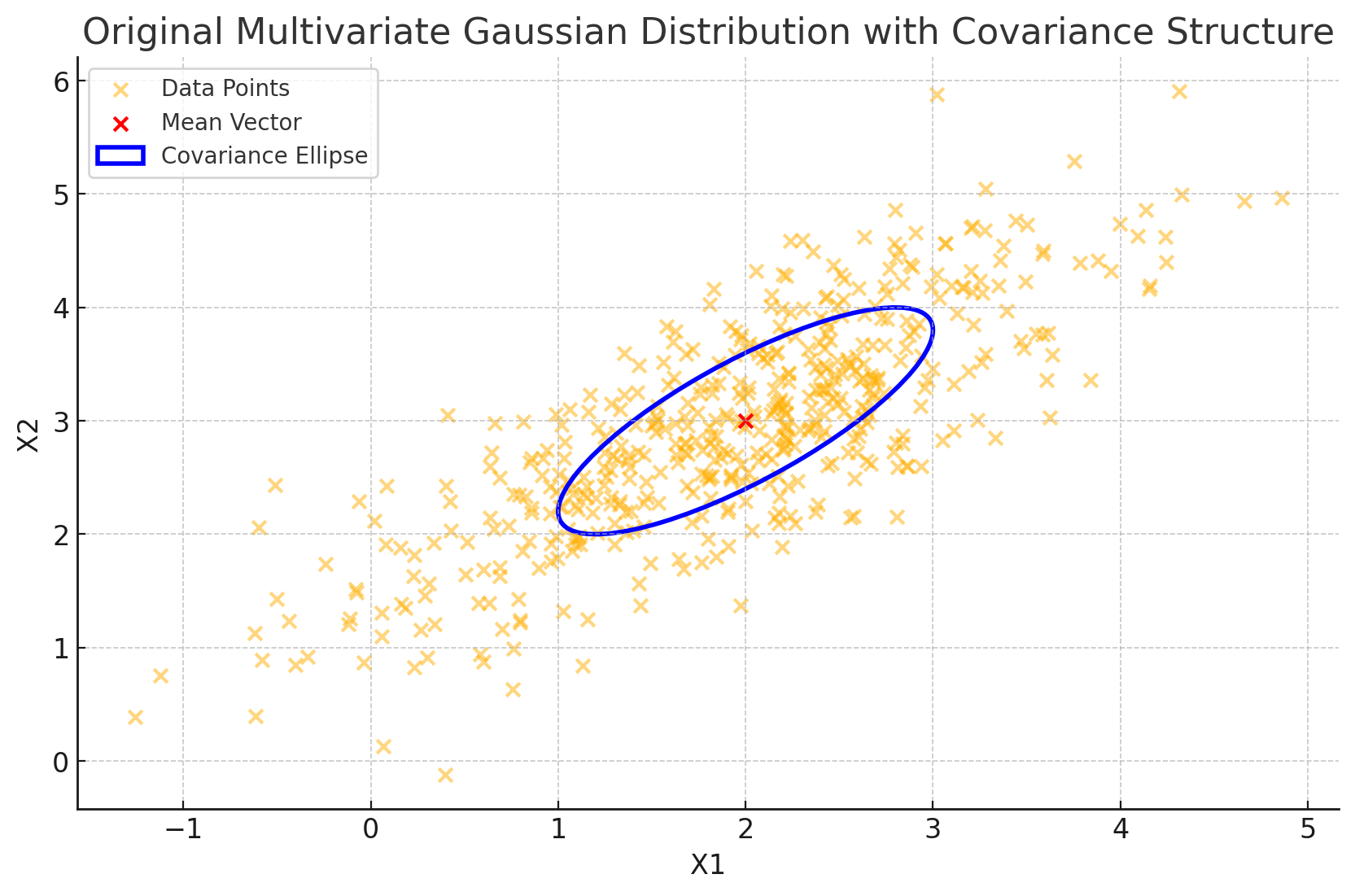
In this example, we’ll use the same mean vector \(\mu = \begin{bmatrix} 2 \\ 3 \end{bmatrix}\) and a covariance matrix \(\Sigma = \begin{bmatrix} 1 & 0.8 \\ 0.8 & 1 \end{bmatrix}\). The positive off-diagonal values indicate a positive correlation between the two variables, meaning they tend to vary together.

import numpy as np
import matplotlib.pyplot as plt

# Define the mean vector and covariance matrix
mu = np.array([2, 3])
cov = np.array([[1, 0.8], [0.8, 1]])

# Generate data points from a 2D Gaussian distribution
data = np.random.multivariate_normal(mu, cov, 500)

# Plot the data cloud and the covariance structure
plt.figure(figsize=(10, 6))
plt.scatter(data[:, 0], data[:, 1], alpha=0.5, label='Data Points')
plt.scatter(mu[0], mu[1], color='red', marker='x', label='Mean Vector')
plt.xlabel('X1')
plt.ylabel('X2')
plt.title('Original Multivariate Gaussian Distribution with Covariance Structure')
plt.legend()

# Visualize the covariance as an ellipse
from matplotlib.patches import Ellipse

# Eigenvalues and eigenvectors of the covariance matrix
eigvals, eigvecs = np.linalg.eigh(cov)
angle = np.degrees(np.arctan2(*eigvecs[:,0][::-1]))

# Width and height of the ellipse based on the eigenvalues (scaled for visibility)
width, height = 2 * np.sqrt(eigvals)
ellipse = Ellipse(xy=mu, width=width, height=height, angle=angle, edgecolor='blue', fc='None', lw=2, label='Covariance Ellipse')
plt.gca().add_patch(ellipse)
plt.legend()
plt.show()

In this code, we:

1. Generate a data cloud based on \(\Sigma\), capturing the positive correlation between \(X_1\) and \(X_2\).
2. Plot the data points along with the mean vector.
3. Use the eigenvalues and eigenvectors of \(\Sigma\) to plot an ellipse representing the covariance structure. The orientation and size of this ellipse reflect the spread and correlation encoded in \(\Sigma\), with the longer axis aligned along the direction of greatest variance.

Step 2: Apply a Linear Transformation and Observe the Covariance Matrix Change

Next, let’s apply a linear transformation to our data. We’ll use a transformation matrix \(A = \begin{bmatrix} 1.2 & 0.5 \\ 0.3 & 0.8 \end{bmatrix}\), which will stretch and rotate the data. According to our earlier derivation, the new covariance matrix should be \(A \Sigma A^T\).

# Define the transformation matrix A
A = np.array([[1.2, 0.5], [0.3, 0.8]])

# Transform the data
transformed_data = data @ A.T

# Calculate the transformed covariance matrix
transformed_cov = A @ cov @ A.T

# Plot the transformed data and new covariance structure
plt.figure(figsize=(10, 6))
plt.scatter(transformed_data[:, 0], transformed_data[:, 1], alpha=0.5, label='Transformed Data Points')
plt.xlabel('Y1')
plt.ylabel('Y2')
plt.title('Transformed Multivariate Gaussian Distribution with New Covariance Structure')

# Calculate and plot the new covariance ellipse
eigvals, eigvecs = np.linalg.eigh(transformed_cov)
angle = np.degrees(np.arctan2(*eigvecs[:,0][::-1]))
width, height = 2 * np.sqrt(eigvals)
ellipse = Ellipse(xy=A @ mu, width=width, height=height, angle=angle, edgecolor='green', fc='None', lw=2, label='Transformed Covariance Ellipse')
plt.gca().add_patch(ellipse)
plt.legend()
plt.show()

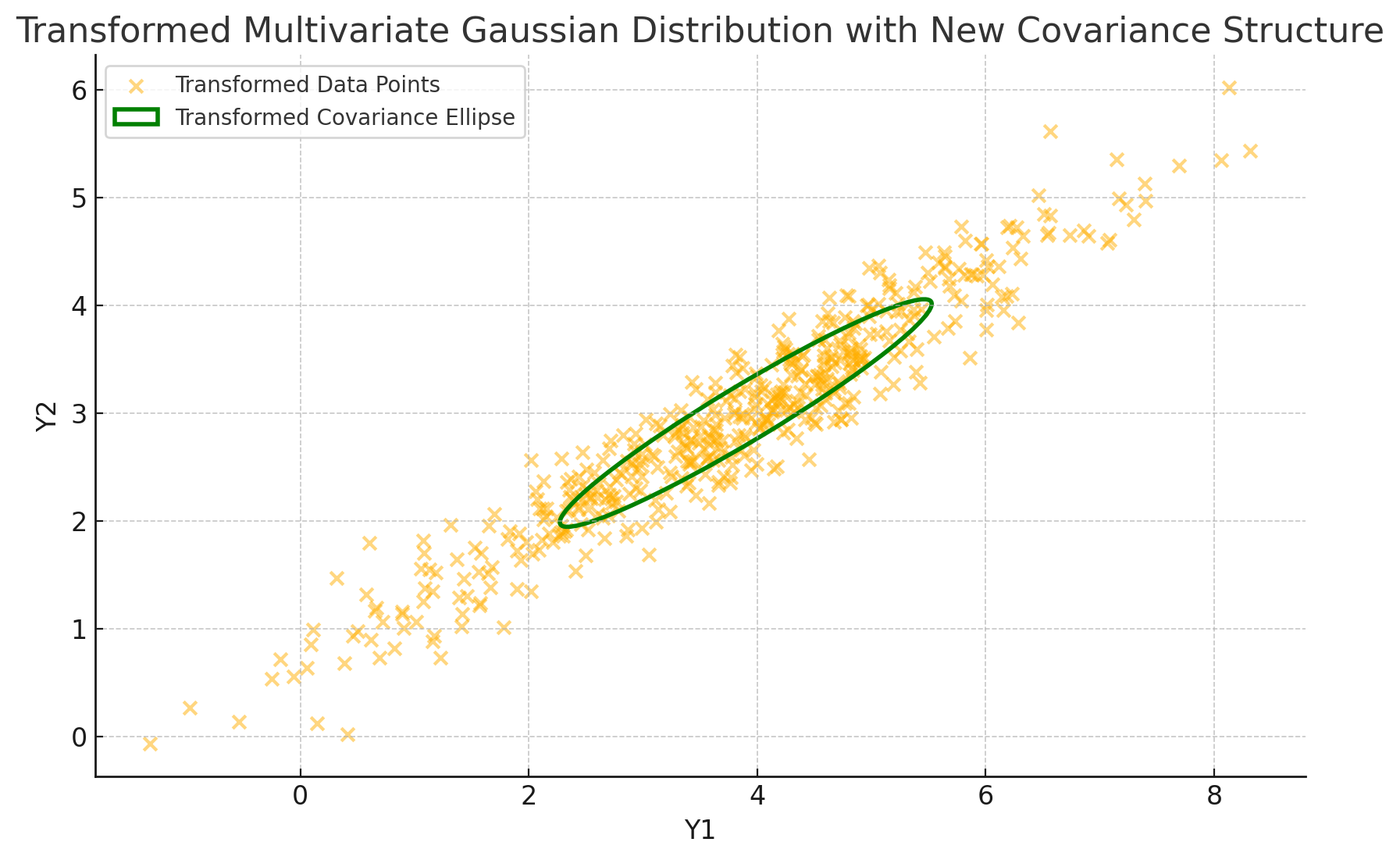
In this visualization:

1. We transform the data by applying \(A\), which stretches and rotates the original distribution.
2. We compute the transformed covariance matrix as \(A \Sigma A^T\) and plot the new covariance ellipse to represent its structure.

Observations

With this code, we see the impact of a linear transformation on the covariance matrix:

• Spread and Orientation: The transformed covariance ellipse is reshaped and reoriented. The principal axes of the ellipse align with the directions of greatest and least variance in the transformed data, which reflect the new covariance structure encoded by \(A \Sigma A^T\).
• Predicted Transformation: The calculation \(A \Sigma A^T\) matches the new spread, showing that even though the data has shifted in space, we can predict exactly how its variability changes.

The Geometric Meaning of the Covariance Matrix

At this point, we know the covariance matrix \(\Sigma\) defines the structure of a multivariate Gaussian distribution in terms of variance and covariance. But what does \(\Sigma\) really look like? In a two-dimensional space, the covariance matrix paints an elegant picture of geometry, describing a distribution’s shape as an ellipse. This section is a journey into the geometric implications of \(\Sigma\), where each feature of the covariance matrix corresponds to a unique aspect of the data’s spatial spread.

Elliptical Contours: The Shape of Data in 2D

In the case of a two-dimensional Gaussian distribution, the contours of equal density—think of these as the “outlines” or “borders” where data points tend to cluster—form concentric ellipses. These ellipses reveal the spread of data around the mean vector \(\mu\) and are directly determined by the covariance matrix \(\Sigma\).

Each ellipse’s geometry—the length and direction of its axes—offers a visual interpretation of \(\Sigma\):

1. Principal Axes (Direction): The directions of the ellipse’s axes correspond to the eigenvectors of \(\Sigma\). These eigenvectors are vectors in space that point along the directions where the data varies the most (the “principal directions”).
2. Axis Lengths (Spread): The lengths of these axes are proportional to the square roots of the eigenvalues of \(\Sigma\). The larger an eigenvalue, the longer the axis, meaning that data stretches more along this direction. Smaller eigenvalues correspond to shorter axes, indicating less variability in that direction.

Eigenvalue Decomposition of the Covariance Matrix

To understand the ellipse’s structure more deeply, let’s look at the eigenvalue decomposition of \(\Sigma\). The covariance matrix \(\Sigma\) is symmetric, meaning it can be decomposed as:

where:

• \(Q\) is a matrix of eigenvectors of \(\Sigma\), and
• \(\Lambda\) is a diagonal matrix of eigenvalues of \(\Sigma\), with each eigenvalue corresponding to the variance along a principal direction.

This decomposition provides a clean geometric interpretation. If we rewrite our multivariate random variable \(X\) (centered at the origin for simplicity) as:

where \(D = \sqrt{\Lambda}\) is the matrix of square roots of the eigenvalues and \(Z\) is a vector of standard normal variables, we can see that \(Q\) rotates the data along the principal directions and \(D\) scales it according to the variances.

Let’s illustrate this in two steps.

Step 1: Visualize the Original Data with Eigenvectors

We can start by plotting the original data and overlaying the eigenvectors of \(\Sigma\) to visualize the principal directions.

import numpy as np
import matplotlib.pyplot as plt

# Define mean and covariance matrix
mu = np.array([2, 3])
cov = np.array([[3, 1], [1, 2]])

# Generate data
data = np.random.multivariate_normal(mu, cov, 500)

# Plot the data
plt.figure(figsize=(10, 6))
plt.scatter(data[:, 0], data[:, 1], alpha=0.5, label='Data Points')
plt.scatter(mu[0], mu[1], color='red', marker='x', label='Mean Vector')
plt.xlabel('X1')
plt.ylabel('X2')
plt.title('Multivariate Gaussian with Principal Directions')

# Compute eigenvalues and eigenvectors
eigvals, eigvecs = np.linalg.eigh(cov)

# Plot eigenvectors as principal directions
for i in range(len(eigvals)):
    plt.plot([mu[0], mu[0] + np.sqrt(eigvals[i]) * eigvecs[0, i]],
             [mu[1], mu[1] + np.sqrt(eigvals[i]) * eigvecs[1, i]],
             label=f'Principal Direction {i+1}', linewidth=2)

plt.legend()
plt.show()

In this code, we:

1. Generate data according to the mean \(\mu\) and covariance matrix \(\Sigma\).
2. Plot the data along with the mean vector.
3. Compute the eigenvalues and eigenvectors of \(\Sigma\), and overlay the eigenvectors on the data, scaled by the square root of their corresponding eigenvalues to represent the primary directions and spread.

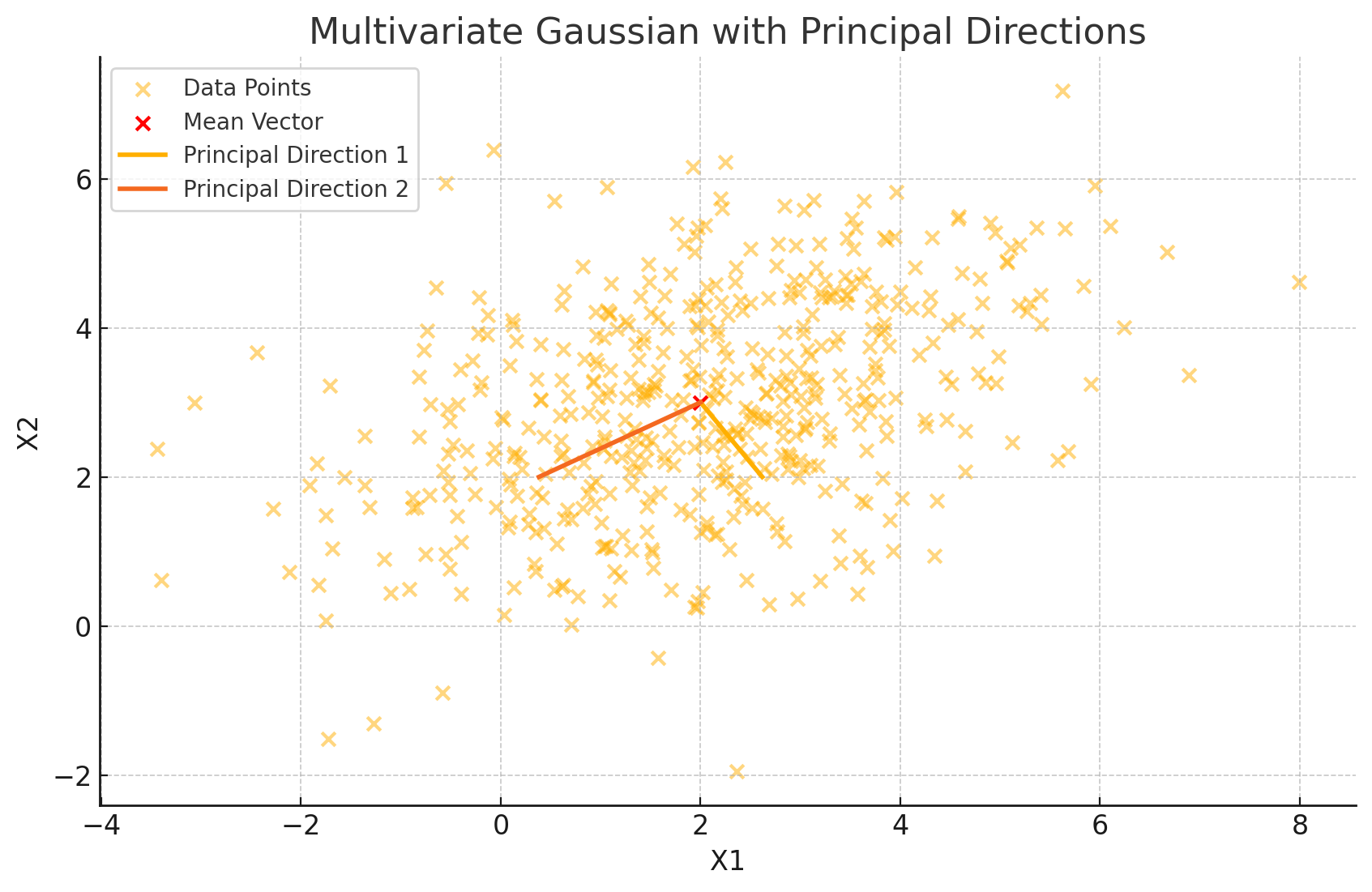
The eigenvectors point along the primary axes of the data, while their lengths, scaled by the square roots of the eigenvalues, indicate how far the data stretches along these axes. This visualization immediately tells us the directions in which our data is most (or least) spread out.

Step 2: Visualizing the Covariance Matrix as an Ellipse

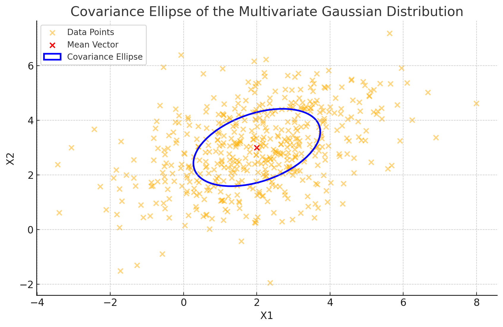
To highlight the covariance structure even further, we can draw the ellipse representing a particular level set of our Gaussian density. Here’s the code to do so, using the eigenvalues and eigenvectors to construct an ellipse around the data:

# Plot data with covariance ellipse
plt.figure(figsize=(10, 6))
plt.scatter(data[:, 0], data[:, 1], alpha=0.5, label='Data Points')
plt.scatter(mu[0], mu[1], color='red', marker='x', label='Mean Vector')
plt.xlabel('X1')
plt.ylabel('X2')
plt.title('Covariance Ellipse of the Multivariate Gaussian Distribution')

# Draw the ellipse
from matplotlib.patches import Ellipse
angle = np.degrees(np.arctan2(*eigvecs[:,0][::-1]))
width, height = 2 * np.sqrt(eigvals)  # Ellipse axes scaled to represent variance
ellipse = Ellipse(xy=mu, width=width, height=height, angle=angle, edgecolor='blue', fc='None', lw=2, label='Covariance Ellipse')
plt.gca().add_patch(ellipse)

plt.legend()
plt.show()

This plot gives us a clear visual representation of the covariance matrix’s “footprint” on the data:

• Direction: The ellipse’s major and minor axes correspond to the principal directions (eigenvectors) of the data spread.
• Length of Axes: The lengths of these axes are proportional to the square roots of the eigenvalues of \(\Sigma\), indicating the variance along each direction.

Geometric Takeaways

So, what does this ellipse tell us about the data’s geometry?

1. Primary Spread: The major axis shows where the data is most dispersed, aligned along the eigenvector with the largest eigenvalue. This direction represents the direction of greatest variance.
2. Secondary Spread: The minor axis, perpendicular to the major axis, aligns with the eigenvector of the smaller eigenvalue, showing where the data is more tightly clustered.

This elliptical geometry offers a powerful intuition: the covariance matrix defines an oriented and scaled ellipse that encapsulates the data’s spread and directionality. By examining this shape, we can quickly grasp the underlying structure of the distribution—its direction of spread, symmetry (or lack thereof), and how tightly data points are packed.

A Practical Example of Deriving the Covariance Matrix

To ground our understanding of the covariance matrix in something concrete, let’s work through a hands-on example. We’ll take a simple two-dimensional random variable, calculate its mean vector and covariance matrix from a small dataset, and observe how these values summarize our data.

Imagine we have a dataset representing the measurements of two variables, say \(X_1\) and \(X_2\), for simplicity. This could be anything—a set of financial returns, height and weight pairs, or temperatures at different locations. Let’s define our random variable \(X\) as:

We’ll calculate the sample mean vector \(\hat{\mu}\) and the sample covariance matrix \(\hat{\Sigma}\) based on observed data.

Step 1: Calculate the Sample Mean Vector

Let’s start with the sample mean vector, which captures the “central location” of the data. Given \(N\) observations, we define the sample mean \(\hat{\mu}\) as:

where \(X_i\) represents the \(i\)-th observation of our random variable \(X\).

For instance, suppose we have the following five observations:

The sample mean vector \(\hat{\mu}\) is then calculated as:

Breaking it down component-wise:

Thus, our mean vector is:

Step 2: Calculate the Sample Covariance Matrix

Next, let’s calculate the sample covariance matrix, which tells us not only the variability of each variable but also how \(X_1\) and \(X_2\) move in relation to each other. The sample covariance matrix \(\hat{\Sigma}\) is defined as:

For our five observations, \(N = 5\), so we’ll divide by \(4\) (that’s \(N - 1\)).

Let’s compute each term \((X_i - \hat{\mu})(X_i - \hat{\mu})^T\) for each observation:

1. For \(X_1 = \begin{bmatrix} 2 \\ 3 \end{bmatrix}\):

   \[X_1 - \hat{\mu} = \begin{bmatrix} 2 \\ 3 \end{bmatrix} - \begin{bmatrix} 4.8 \\ 6.6 \end{bmatrix} = \begin{bmatrix} -2.8 \\ -3.6 \end{bmatrix},\]

   and

   \[(X_1 - \hat{\mu})(X_1 - \hat{\mu})^T = \begin{bmatrix} -2.8 \\ -3.6 \end{bmatrix} \begin{bmatrix} -2.8 & -3.6 \end{bmatrix} = \begin{bmatrix} 7.84 & 10.08 \\ 10.08 & 12.96 \end{bmatrix}.\]

2. For \(X_2 = \begin{bmatrix} 3 \\ 5 \end{bmatrix}\):

   \[X_2 - \hat{\mu} = \begin{bmatrix} 3 \\ 5 \end{bmatrix} - \begin{bmatrix} 4.8 \\ 6.6 \end{bmatrix} = \begin{bmatrix} -1.8 \\ -1.6 \end{bmatrix},\]

   and

   \[(X_2 - \hat{\mu})(X_2 - \hat{\mu})^T = \begin{bmatrix} -1.8 \\ -1.6 \end{bmatrix} \begin{bmatrix} -1.8 & -1.6 \end{bmatrix} = \begin{bmatrix} 3.24 & 2.88 \\ 2.88 & 2.56 \end{bmatrix}.\]

3. For \(X_3 = \begin{bmatrix} 5 \\ 7 \end{bmatrix}\):

   \[X_3 - \hat{\mu} = \begin{bmatrix} 5 \\ 7 \end{bmatrix} - \begin{bmatrix} 4.8 \\ 6.6 \end{bmatrix} = \begin{bmatrix} 0.2 \\ 0.4 \end{bmatrix},\]

   and

   \[(X_3 - \hat{\mu})(X_3 - \hat{\mu})^T = \begin{bmatrix} 0.2 \\ 0.4 \end{bmatrix} \begin{bmatrix} 0.2 & 0.4 \end{bmatrix} = \begin{bmatrix} 0.04 & 0.08 \\ 0.08 & 0.16 \end{bmatrix}.\]

4. For \(X_4 = \begin{bmatrix} 6 \\ 8 \end{bmatrix}\):

   \[X_4 - \hat{\mu} = \begin{bmatrix} 6 \\ 8 \end{bmatrix} - \begin{bmatrix} 4.8 \\ 6.6 \end{bmatrix} = \begin{bmatrix} 1.2 \\ 1.4 \end{bmatrix},\]

   and

   \[(X_4 - \hat{\mu})(X_4 - \hat{\mu})^T = \begin{bmatrix} 1.2 \\ 1.4 \end{bmatrix} \begin{bmatrix} 1.2 & 1.4 \end{bmatrix} = \begin{bmatrix} 1.44 & 1.68 \\ 1.68 & 1.96 \end{bmatrix}.\]

5. For \(X_5 = \begin{bmatrix} 8 \\ 10 \end{bmatrix}\): \(X_5 - \hat{\mu} = \begin{bmatrix} 8 \\ 10 \end{bmatrix} - \begin{bmatrix} 4.8 \\ 6.6 \end{bmatrix} = \begin{bmatrix} 3.2 \\ 3.4 \end{bmatrix},\) and \((X_5 - \hat{\mu})(X_5 - \hat{\mu})^T = \begin{bmatrix} 3.2 \\ 3.4 \end{bmatrix} \begin{bmatrix} 3.2 & 3.4 \end{bmatrix} = \begin{bmatrix} 10.24 & 10.88 \\ 10.88 & 11.56 \end{bmatrix}.\)

Now, we add these matrices and divide by \(N - 1 = 4\) to get the sample covariance matrix:

After summing the matrices:

Summary

In this example, we’ve calculated both the sample mean vector and the sample covariance matrix. Our sample covariance matrix, \(\hat{\Sigma} = \begin{bmatrix} 5.7 & 6.4 \\ 6.4 & 7.3 \end{bmatrix}\), encapsulates the spread and relationship between \(X_1\) and \(X_2\). The off-diagonal terms (6.4) represent the covariance between \(X_1\) and \(X_2\), indicating a positive correlation, while the diagonal terms represent the variances of \(X_1\) and \(X_2\) individually.

This simple calculation reinforces the power of the covariance matrix—it captures both the “spread” of each variable and their interaction, providing a complete picture of our data’s geometric and statistical structure.

Covariance Matrix and Independence

As we wrap up our journey into the world of covariance matrices, it’s fitting to address one of the most common misconceptions: the relationship between independence and uncorrelatedness. In the world of multivariate distributions, understanding whether two variables are independent or merely uncorrelated is crucial. The covariance matrix can give us valuable insights, but it has its limitations—especially when it comes to verifying true independence.

Defining Independence

In probability theory, two random variables \(X_i\) and \(X_j\) are defined to be independent if the occurrence of one has no influence on the probability distribution of the other. Mathematically, this means:

for all \(x\) and \(y\). In simpler terms, knowing the value of \(X_i\) provides no information about \(X_j\) and vice versa.

Covariance and Independence: A Subtle Distinction

The covariance matrix tells us about the linear relationships between variables, but not necessarily about their independence. For two variables \(X_i\) and \(X_j\), the covariance \(\text{Cov}(X_i, X_j)\) is defined as:

If \(X_i\) and \(X_j\) are independent, then \(\text{Cov}(X_i, X_j) = 0\). Independence implies that there is no relationship between the variables at all, which includes a lack of linear correlation. However, the reverse is not true: zero covariance does not imply independence.

To see why, let’s explore this distinction mathematically and with an example.

Proof that Zero Covariance Does Not Imply Independence

To understand why zero covariance does not necessarily mean independence, consider two random variables \(X\) and \(Y\) that are uncorrelated (i.e., \(\text{Cov}(X, Y) = 0\)) but not independent.

Let \(X\) be a standard normal random variable: \(X \sim N(0, 1)\). Now define \(Y = X^2\). Clearly, \(Y\) depends on \(X\); in fact, \(Y\) is entirely determined by \(X\), so \(X\) and \(Y\) are not independent.

1. Calculating the Covariance: We’ll calculate \(\text{Cov}(X, Y)\) to see if they’re uncorrelated.

   \[\text{Cov}(X, Y) = E[(X - E[X])(Y - E[Y])].\]

   Since \(X \sim N(0, 1)\), we have \(E[X] = 0\) and \(E[Y] = E[X^2] = \text{Var}(X) = 1\). So,

   \[\text{Cov}(X, Y) = E[X(Y - 1)] = E[X(X^2 - 1)] = E[X^3 - X].\]

2. Expectation of Odd Moments: Given that \(X\) is normally distributed with mean 0, all odd moments of \(X\) (such as \(E[X]\) and \(E[X^3]\)) are zero. Therefore,

   \[\text{Cov}(X, Y) = E[X^3] - E[X] = 0 - 0 = 0.\]

   Thus, \(\text{Cov}(X, Y) = 0\), indicating that \(X\) and \(Y\) are uncorrelated. But as we know, \(Y = X^2\), which is entirely determined by \(X\). Therefore, they are not independent, even though they are uncorrelated.

This example highlights a key takeaway: uncorrelated variables are not necessarily independent. Covariance only captures linear relationships, so two variables could have a non-linear dependency and still exhibit zero covariance.

Role of the Covariance Matrix in Independence Analysis

The covariance matrix \(\Sigma\) provides us with a way to examine linear dependencies between variables. Each off-diagonal element \(\Sigma\_{ij} = \text{Cov}(X_i, X_j)\) indicates the extent to which two variables vary together. If all off-diagonal entries of \(\Sigma\) are zero, we know that each pair of variables is uncorrelated. However, this does not guarantee independence.

For multivariate normal distributions, however, the story is simpler. In a multivariate normal distribution, uncorrelated variables are indeed independent. Specifically, if \(X \sim N(\mu, \Sigma)\), then zero off-diagonal entries in \(\Sigma\) imply that the components of \(X\) are independent. This is a special property of the Gaussian distribution and does not hold in general.

Practical Implications

When analyzing real-world data, it’s essential to remember that zero covariance should not be mistaken for independence unless you’re specifically working with a multivariate Gaussian. In most other cases, zero covariance merely indicates a lack of linear relationship. Non-linear dependencies, which are common in fields like finance, biology, and machine learning, can often “hide” behind zero covariance.

In summary, the covariance matrix is a powerful tool for understanding linear relationships but is limited in detecting true independence. When we need a full assessment of independence, especially in non-Gaussian contexts, we have to look beyond \(\Sigma\) and consider additional techniques, such as analyzing joint distributions or using tests for independence.

Conclusion

The mean vector serves as the “center of gravity” for the data, shifting predictably under transformations and providing a concise summary of central tendencies across dimensions. Meanwhile, the covariance matrix is a lens into the data’s geometry. It encodes not only the individual variances of each variable but also the pairwise interactions that reveal whether variables rise and fall together or act independently. This matrix’s symmetry and positive semi-definiteness give it a unique role in shaping data contours and helping analysts visualize distribution shape, orientation, and spread.

But as we’ve seen, the covariance matrix also has its limits. While it efficiently captures linear relationships, it cannot capture the entire complexity of data dependencies. As our exploration of independence versus uncorrelatedness shows, true independence requires more than just a zero covariance—especially in non-Gaussian settings where nonlinear dependencies can lie hidden. Understanding these nuances is crucial for effective data analysis. In real-world applications, whether in finance, biology, or machine learning, knowing when the covariance matrix can (and cannot) tell the full story allows us to apply these tools more accurately and creatively.