A Sketch of Proofs for Some Properties of Multivariate Gaussian Distribution

Introduction

In the previous blog post, we discussed the extension from univariate to multivariate Gaussian distributions and examined the transformation in their functional form. Moving from a single variable to an N-dimensional space introduces a rich structure where properties like independence, marginal distributions, and conditional behaviors play a crucial role in understanding the multivariate Gaussian distribution in depth. In this post, we will provide a sketch of proofs for several key properties of multivariate Gaussians. These properties include the independence of Gaussian random vectors, the derivation of marginal and conditional distributions, the invariance of covariance under transformations, and the behavior of Gaussian distributions under linear transformations. Rather than delving into detailed, rigorous proofs, we aim to offer an intuitive and accessible overview, highlighting the underlying mathematical concepts without overwhelming technical detail.

Proving the Independence of Gaussian Random Vectors

The relationship between the covariance structure of a random vector and its independence properties plays a key role in many machine learning algorithms, signal processing, and other applied fields. It is particularly relevant in Gaussian processes, where we assume that the random vectors representing function values are often independent, under certain conditions. So, let’s break down the problem mathematically, focusing on proving the independence of the components of a multivariate Gaussian vector. The path to this insight involves linear algebra, specifically understanding the covariance matrix and its diagonalization.

Covariance Matrix Diagonalization and Independence

Consider a random vector \(\mathbf{X} = (X_1, X_2, \dots, X_k)^T\) following a multivariate normal distribution with mean vector \(\mu = (\mu_1, \mu_2, \dots, \mu_k)^T\) and covariance matrix \(\Sigma\).

The probability density function (PDF) of this multivariate Gaussian distribution is given by:

Here, \(\Sigma\) is a \(k \times k\) covariance matrix, where the diagonal elements \(\sigma_i^2\) represent the variances of each component of the vector \(\mathbf{X}\), and the off-diagonal elements \(\sigma_{ij}\) represent the covariances between the components \(X_i\) and \(X_j\).

Now, to examine the independence of the components of \(\mathbf{X}\), we need to focus on the structure of the covariance matrix \(\Sigma\). For random variables to be independent, their covariance must be zero. This leads to the crucial fact that if the covariance matrix is diagonal, then the components of \(\mathbf{X}\) must be independent. The question now is: when does this happen?

Diagonalization of Covariance Matrix

We know from linear algebra that any symmetric matrix, including the covariance matrix \(\Sigma\), can be diagonalized by an orthogonal transformation. This means that there exists an orthogonal matrix \(Q\) (i.e., \(Q^T Q = I\)) such that:

where \(D\) is a diagonal matrix. Each diagonal element of \(D\), say \(\sigma_i^2\), corresponds to the variance of the transformed variables, which are linear combinations of the original components of \(\mathbf{X}\).

To unpack this geometrically: the matrix \(Q\) represents a rotation (or possibly reflection) of the coordinate axes in the space of the random vector \(\mathbf{X}\). After the transformation, the random vector \(\mathbf{Y} = Q^T \mathbf{X}\) will have components \(Y_1, Y_2, \dots, Y_k\), each with variance \(\sigma_i^2\), and no covariances between them. In other words, these transformed components are uncorrelated.

But here’s the critical point: uncorrelated components in a multivariate normal distribution are independent. This result holds because the multivariate normal distribution has a special property: if its components are uncorrelated, they must also be independent. This follows from the fact that the joint distribution factorizes when the covariance matrix is diagonal.

Formal Proof of Independence

Let’s now formalize this with a rigorous proof. Given that the covariance matrix \(\Sigma\) is diagonal, it can be written as:

The off-diagonal elements of \(\Sigma\) are zero, indicating that the components of \(\mathbf{X}\) are uncorrelated.

For two random variables \(X_i\) and \(X_j\), their covariance is defined as:

If the covariance matrix \(\Sigma\) is diagonal, then:

This implies that \(X_i\) and \(X_j\) are uncorrelated. Since we are dealing with a multivariate normal distribution, this uncorrelation implies that \(X_i\) and \(X_j\) are independent.

Thus, if the covariance matrix \(\Sigma\) is diagonal, the components of \(\mathbf{X}\) are independent, and we can conclude:

Geometrical Intuition

To gain some geometrical intuition, think of a random vector \(\mathbf{X}\) in a high-dimensional space. The covariance matrix \(\Sigma\) captures how the components of \(\mathbf{X}\) vary together. If the covariance matrix is diagonal, this indicates that the components of \(\mathbf{X}\) do not “mix” with one another—they vary independently along different directions of the space.

When we diagonalize the covariance matrix, we essentially rotate the space such that the axes align with the principal directions of variation. Along each axis, the corresponding component of \(\mathbf{X}\) varies independently of the others. This geometric interpretation aligns with the algebraic fact that the components are independent when the covariance matrix is diagonal.

Demo

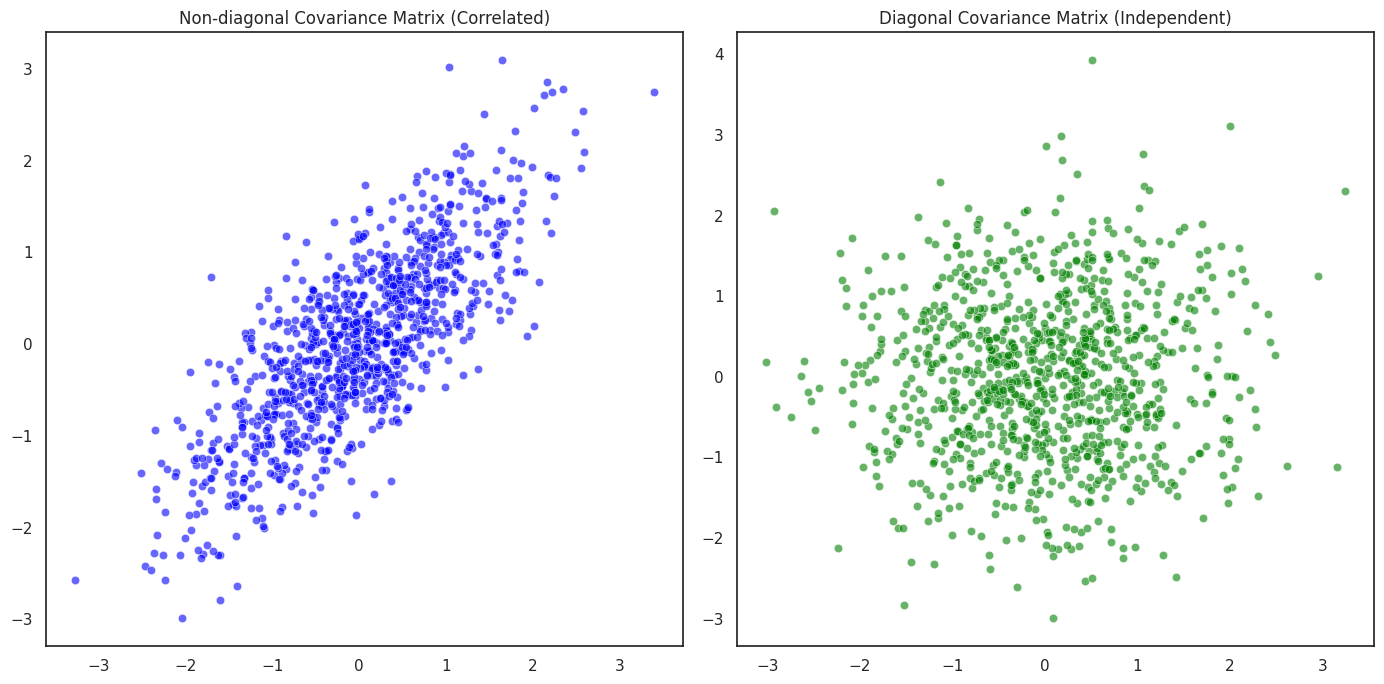
In this section, we explore how the covariance matrix influences the distribution of multivariate Gaussian random variables. Specifically, we’ll visualize the difference between correlated and independent random variables by examining two different covariance matrices: one that introduces correlation between the components and one that enforces independence.

We will work with a bivariate Gaussian distribution, where the random vector \(\mathbf{x} = [X_1, X_2]^T\) has a mean vector \(\mu = [0, 0]^T\). The covariance matrix determines the shape and orientation of the distribution in the feature space.

1. Non-diagonal Covariance Matrix (Correlated Case): A covariance matrix with off-diagonal elements (non-zero values) implies that the two components \(X_1\) and \(X_2\) are correlated. For example, a covariance matrix like:

   \[\Sigma = \begin{bmatrix} 1 & 0.8 \\ 0.8 & 1 \end{bmatrix}\]

   indicates a positive correlation between \(X_1\) and \(X_2\). When plotted, this produces an elliptical distribution, where the data points are spread in a specific direction, showing a linear relationship between the two variables.

2. Diagonal Covariance Matrix (Independent Case): A diagonal covariance matrix implies that the two variables are independent. For example:

   \[\Sigma = \begin{bmatrix} 1 & 0 \\ 0 & 1 \end{bmatrix}\]

   In this case, there is no correlation between \(X_1\) and \(X_2\), and the distribution is circular. The points are spread equally in all directions, showing no linear dependence between the two variables.

import numpy as np
import seaborn as sns
import matplotlib.pyplot as plt

# Set plotting style
sns.set(style="white", palette="muted")

# Seed for reproducibility
np.random.seed(42)

# Define mean and covariance matrices
mean = [0, 0]

# Covariance Matrix 1 (Non-diagonal, correlated)
cov_1 = [[1, 0.8], [0.8, 1]]

# Covariance Matrix 2 (Diagonal, independent)
cov_2 = [[1, 0], [0, 1]]

# Generate random samples
data_1 = np.random.multivariate_normal(mean, cov_1, 1000)
data_2 = np.random.multivariate_normal(mean, cov_2, 1000)

# Plotting the samples
fig, ax = plt.subplots(1, 2, figsize=(14, 7))

# Plotting the non-diagonal covariance samples
sns.scatterplot(x=data_1[:, 0], y=data_1[:, 1], ax=ax[0], color="blue", alpha=0.6)
ax[0].set_title("Non-diagonal Covariance Matrix (Correlated)")

# Plotting the diagonal covariance samples
sns.scatterplot(x=data_2[:, 0], y=data_2[:, 1], ax=ax[1], color="green", alpha=0.6)
ax[1].set_title("Diagonal Covariance Matrix (Independent)")

plt.tight_layout()
plt.show()

1. Non-diagonal Covariance Matrix (Correlated Case): In the first plot (left), where the covariance matrix contains off-diagonal values (0.8), the points form an elongated ellipse. This shows that the two variables \(X_1\) and \(X_2\) are positively correlated. The data points are not spread equally in all directions but rather along the principal axes of the ellipse, which reflects the dependency between the variables.

2. Diagonal Covariance Matrix (Independent Case): In the second plot (right), the covariance matrix is diagonal, indicating that \(X_1\) and \(X_2\) are independent. The points form a circular distribution, with no discernible directionality. This indicates that the changes in \(X_1\) do not depend on \(X_2\), and vice versa. The variables are independent, which is precisely what the diagonal covariance structure represents.

Deriving Marginal and Conditional Distributions of Multivariate Gaussians

The fact that while the marginal distributions of a multivariate Gaussian are always Gaussian, the reverse inference is not true.

Deriving the Marginal Distribution

In probability theory, the marginal distribution is the distribution of a subset of variables, ignoring the others. Mathematically, for a random vector \(\mathbf{X} = [X_1, X_2, \dots, X_k]^T\) following a multivariate Gaussian distribution with mean vector \(\mu = [\mu_1, \mu_2, \dots, \mu_k]^T\) and covariance matrix \(\Sigma\), the marginal distribution of a subset of the components of \(\mathbf{X}\) is still a Gaussian distribution.

Suppose we have a partition of the vector \(\mathbf{X}\) into two disjoint subsets: \(\mathbf{X}_S\) (the subset of interest) and \(\mathbf{X}_C\) (the complement of \(\mathbf{X}_S\)).

The full vector \(\mathbf{X}\) follows a multivariate normal distribution:

We want to derive the marginal distribution of \(\mathbf{X}_S\), i.e., the distribution of just the subset \(\mathbf{X}_S\) while marginalizing over the components of \(\mathbf{X}_C\). The marginal distribution is obtained by integrating out the components corresponding to \(\mathbf{X}_C\) from the joint distribution.

The joint PDF of \(\mathbf{X}\) is given by:

Now, let’s partition the mean vector \(\mu\) and the covariance matrix \(\Sigma\) as follows:

Where:

• \(\mu_S\) is the mean vector for the subset \(\mathbf{X}_S\),
• \(\mu_C\) is the mean vector for the complement \(\mathbf{X}_C\),
• \(\Sigma_{SS}\) is the covariance matrix between the components in \(\mathbf{X}_S\),
• \(\Sigma_{SC}\) and \(\Sigma_{CS}\) are the cross-covariances between \(\mathbf{X}_S\) and \(\mathbf{X}_C\),
• \(\Sigma_{CC}\) is the covariance matrix of \(\mathbf{X}_C\).

To find the marginal distribution of \(\mathbf{X}_S\), we integrate out the complement \(\mathbf{X}_C\) from the joint PDF. That is we compute the integral:

Substituting the partitioned PDF:

This integral can be solved, and the result is another Gaussian distribution for \(\mathbf{x}_S\), with mean \(\mu_S\) and covariance matrix \(\Sigma_{SS}\):

Thus, the marginal distribution of \(\mathbf{X}_S\) is still Gaussian, as expected.

Reverse Inference: Marginal Distributions Do Not Imply Multivariate Normality

While it is clear from the above derivation that the marginal distribution of any subset of a multivariate Gaussian is also Gaussian, there is an interesting and subtle issue when trying to reverse the argument. That is, just because the marginal distributions of a random vector are Gaussian does not necessarily mean the entire vector follows a multivariate Gaussian distribution.

Suppose we have a random vector \(\mathbf{X} = [X_1, X_2]^T\), and we know that each component \(X_1\) and \(X_2\) is distributed according to a Gaussian distribution:

This implies that the marginal distributions of \(X_1\) and \(X_2\) are Gaussian. However, this does not imply that the joint distribution \((X_1, X_2)\) is necessarily Gaussian. To see this, we need to consider a counterexample.

Counterexample: Suppose that we have two random variables \(X_1\) and \(X_2\) which are both Gaussian marginally, but their joint distribution is not Gaussian. This can occur when their joint distribution involves nonlinear relationships or other higher-order dependencies that are not captured by the marginals alone.

For instance, consider the following joint distribution:

Even though the marginals of \(X_1\) and \(X_2\) are Gaussian, the joint distribution clearly isn’t. This demonstrates that knowing the marginal distributions are Gaussian does not provide sufficient information to conclude that the joint distribution is Gaussian.

In simpler terms: marginal Gaussianity is a necessary but not sufficient condition for the joint distribution to be Gaussian.

Invariance of the Multivariate Gaussian Distribution under Linear Transformations

In this section, we explore a crucial property of the multivariate Gaussian distribution: its invariance under linear transformations.

The Setup: A Multivariate Gaussian Vector

We begin with a random vector \(\mathbf{x}\) that follows a multivariate Gaussian distribution:

Here, \(\mu_x\) is the \(k\)-dimensional mean vector \(\mu_x = [\mu_{x1}, \mu_{x2}, \dots, \mu_{xk}]^T\), \(\Sigma_x\) is the \(k \times k\) covariance matrix \(\Sigma_x = \begin{bmatrix} \sigma_{x1}^2 & \text{Cov}(X_1, X_2) & \dots \\ \end{bmatrix}\).

The PDF of \(\mathbf{x}\) is:

We are interested in how the distribution of \(\mathbf{x}\) transforms when we apply a linear transformation to \(\mathbf{x}\).

The Linear Transformation

Consider a linear transformation of the vector \(\mathbf{x}\) defined by:

Where \(A\) is a \(m \times k\) matrix representing the linear transformation, and \(\mathbf{b}\) represents a \(m\)-dimensional translation vector. \(\mathbf{y}\) is a new random vector, which we seek to analyze. Our goal is to show that \(\mathbf{y}\) is also Gaussian and derive the new mean and covariance matrix of \(\mathbf{y}\).

To do this, we use the fact that the multivariate Gaussian distribution is closed under linear transformations. This means that if \(\mathbf{x} \sim \mathcal{N}(\mu_x, \Sigma_x)\), then the transformed vector \(\mathbf{y}\) will follow a multivariate Gaussian distribution as well, albeit with a different mean and covariance matrix.

Deriving the Mean and Covariance of \(\mathbf{y}\)

Step 1: The New Mean Vector

The mean of \(\mathbf{y}\), denoted \(\mu_y\), can be derived by taking the expectation of \(\mathbf{y} = A\mathbf{x} + \mathbf{b}\):

Since the expectation of \(\mathbf{x}\) is \(\mu_x\), we have:

Thus, the mean vector of \(\mathbf{y}\) is simply the linear transformation of the mean vector of \(\mathbf{x}\), plus the translation vector \(\mathbf{b}\).

Step 2: The New Covariance Matrix

Next, we derive the covariance matrix of \(\mathbf{y}\). The covariance matrix \(\Sigma_y\) of \(\mathbf{y}\) is given by the expected value of the outer product of \(\mathbf{y}\) with itself, minus the outer product of the mean of \(\mathbf{y}\) with itself:

Substituting \(\mathbf{y} = A\mathbf{x} + \mathbf{b}\) into this equation, and noting that \(\mathbb{E}[\mathbf{y}] = \mu_y\), we get:

Since \(\mathbf{b} - \mu_y = 0\) (by definition of \(\mu_y\)), this simplifies to:

Recall that \(\mathbb{E}[\mathbf{x} \mathbf{x}^T] = \Sigma_x\), the covariance matrix of \(\mathbf{x}\). Therefore:

This shows that the covariance matrix of the transformed vector \(\mathbf{y}\) is simply the original covariance matrix \(\Sigma_x\), transformed by the matrix \(A\) and its transpose.

Demo

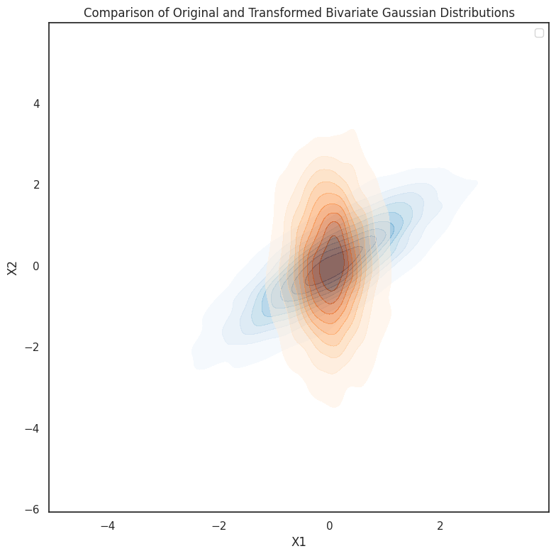
In this experiment, we explore the invariance of multivariate Gaussian distributions under linear transformations. Specifically, we start with a bivariate Gaussian distribution and apply a simple linear transformation, such as rotation, to the data. The transformation is visualized by comparing the original and transformed distributions using scatter plots.

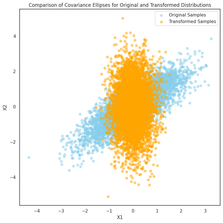
Additionally, we delve into how the covariance structure of the data changes under linear transformations. The covariance ellipses are plotted for both the original and transformed distributions, showing how the shape and orientation of the ellipses reflect the underlying correlations between the variables. This experiment demonstrates that, while the distribution remains Gaussian, the transformation alters the data’s spread and direction,

import numpy as np
import seaborn as sns
import matplotlib.pyplot as plt
import matplotlib.patches as patches

# Set random seed for reproducibility
np.random.seed(0)

# Define original mean and covariance matrix
mu = [0, 0]  # Mean vector
sigma = [[1, 0.8], [0.8, 1]]  # Covariance matrix with positive correlation

# Generate samples from the bivariate Gaussian distribution
x, y = np.random.multivariate_normal(mu, sigma, 5000).T

# Define a simple rotation matrix (45 degrees)
theta = np.pi / 4  # Rotation by 45 degrees
A = np.array([[np.cos(theta), -np.sin(theta)], [np.sin(theta), np.cos(theta)]])
b = np.array([0, 0])  # No translation

# Apply the linear transformation
xy_transformed = np.dot(A, np.vstack([x, y]))  # Perform the linear transformation
xy_transformed = xy_transformed + b[:, np.newaxis]  # Apply the translation vector separately

# Plot the original and transformed distributions on the same axes
fig, ax = plt.subplots(figsize=(8, 8))

# Plot the original distribution with transparency
sns.kdeplot(x=x, y=y, cmap="Blues", fill=True, ax=ax, alpha=0.5, label="Original Distribution")

# Plot the transformed distribution with transparency
sns.kdeplot(x=xy_transformed[0], y=xy_transformed[1], cmap="Oranges", fill=True, ax=ax, alpha=0.5, label="Transformed Distribution")

# Add titles and labels
ax.set_title("Comparison of Original and Transformed Bivariate Gaussian Distributions")
ax.set_xlabel("X1")
ax.set_ylabel("X2")

# Display legend to differentiate the distributions
ax.legend()

plt.tight_layout()
plt.show()

# Function to plot covariance ellipse
def plot_cov_ellipse(covariance, mean, ax, color='blue', label=None):
    # Calculate eigenvalues and eigenvectors
    eigenvalues, eigenvectors = np.linalg.eigh(covariance)
    order = eigenvalues.argsort()[::-1]  # Sort by eigenvalue size
    eigenvalues, eigenvectors = eigenvalues[order], eigenvectors[:, order]
    
    # Calculate rotation angle
    angle = np.degrees(np.arctan2(*eigenvectors[:, 0][::-1]))
    
    # Plot the covariance ellipse
    width, height = 2 * np.sqrt(eigenvalues)
    ell = patches.Ellipse(mean, width, height, angle=angle, color=color, alpha=0.3)
    ax.add_patch(ell)

# Plot covariance ellipses for both distributions on the same axes
fig, ax = plt.subplots(figsize=(8, 8))

# Covariance ellipse for original distribution
plot_cov_ellipse(sigma, mu, ax, color='blue')
ax.scatter(x, y, color='skyblue', alpha=0.5, label="Original Samples")

# Covariance ellipse for transformed distribution
transformed_sigma = A @ sigma @ A.T
plot_cov_ellipse(transformed_sigma, [0, 0], ax, color='orange')
ax.scatter(xy_transformed[0], xy_transformed[1], color='orange', alpha=0.5, label="Transformed Samples")

# Add titles and labels
ax.set_title("Comparison of Covariance Ellipses for Original and Transformed Distributions")
ax.set_xlabel("X1")
ax.set_ylabel("X2")

# Display legend
ax.legend()

plt.tight_layout()
plt.show()

\(\chi^2\) Distribution and the Ellipsoid Theorem

The \(\chi^2\) Distribution: Derivation from Multivariate Gaussian

Let’s begin with the first concept: the \(\chi^2\) distribution. Suppose that \(\mathbf{x} \sim \mathcal{N}(\mu_x, \Sigma_x)\) is a \(k\)-dimensional Gaussian vector, and we are interested in the quadratic form \(Q\):

This expression appears frequently in multivariate statistics, particularly when we are testing hypotheses about the mean vector \(\mu_x\). We’ll show that \(Q\) follows a \(\chi^2\) distribution with \(k\) degrees of freedom.

Step 1: The Transformation to Standard Normal

To analyze \(Q\), we first standardize the vector \(\mathbf{x}\). Let’s consider the transformation \(\mathbf{z} = \Sigma^{-1/2} (\mathbf{x} - \mu_x)\), where \(\Sigma^{-1/2}\) is the matrix square root of \(\Sigma^{-1}\). Under this transformation, \(\mathbf{z}\) follows the standard multivariate normal distribution:

Here, \(I\) is the \(k \times k\) identity matrix. In this new coordinate system, the quadratic form becomes:

Step 2: The \(\chi^2\) Distribution

Now, notice that \(\mathbf{z}^T \mathbf{z}\) is the sum of the squares of \(k\) independent standard normal random variables:

Each \(z_i \sim \mathcal{N}(0,1)\), so \(z_i^2\) follows a \(\chi^2\) distribution with 1 degree of freedom. Thus, the sum of these independent \(\chi^2\) variables, \(Q\), follows a \(\chi^2\) distribution with \(k\) degrees of freedom:

This result tells us that any quadratic form \(\mathbf{x}^T \Sigma^{-1} \mathbf{x}\) in a multivariate Gaussian vector follows a \(\chi^2\) distribution with degrees of freedom equal to the dimensionality of the vector \(\mathbf{x}\).

Demo for the \(\chi^2\) Distribution

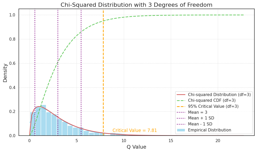
To test this, we simulate 1,000 samples from a 3-dimensional multivariate Gaussian distribution with a mean vector of zeros and an identity covariance matrix. For each sample, we compute the quadratic form \(Q\), which essentially measures the “distance” of each sample from the mean in a scaled manner. By plotting the histogram of these values, we can compare it with the theoretical \(\chi^2\) distribution with 3 degrees of freedom.

The resulting plot includes the simulated distribution of \(Q\), along with the theoretical \(\chi^2\) distribution curve, cumulative distribution function (CDF), the 95% critical value, and markers for the mean and standard deviation.

import numpy as np
import seaborn as sns
import matplotlib.pyplot as plt
from scipy.stats import chi2

# Set experiment parameters
k = 3  # Degrees of freedom, as we are using a 3-dimensional Gaussian
mu = np.zeros(k)  # Mean vector (all zeros)
Sigma = np.eye(k)  # Covariance matrix (identity matrix for simplicity)

# Generate samples from a multivariate normal distribution
np.random.seed(42)  # Set seed for reproducibility
samples = np.random.multivariate_normal(mu, Sigma, 1000)  # 1,000 samples

# Compute the quadratic form Q = x^T * Sigma_inv * x for each sample
Sigma_inv = np.linalg.inv(Sigma)  # Inverse of the covariance matrix
Q = np.sum((samples @ Sigma_inv) * samples, axis=1)  # Quadratic form values

# Plot the histogram of Q values with kernel density estimation (KDE)
plt.figure(figsize=(10, 6))
sns.histplot(Q, kde=True, stat="density", color="skyblue", label="Empirical Distribution", bins=40, alpha=0.7)

# Plot the theoretical Chi-Squared PDF
x = np.linspace(0, np.max(Q), 100)  # Range for theoretical curve
y = chi2.pdf(x, df=k)  # Chi-Squared  PDF with k degrees of freedom
plt.plot(x, y, 'r-', label=f"Chi-squared Distribution (df={k})", linewidth=2)

# Plot the Chi-Squared  CDF for additional reference
y_cdf = chi2.cdf(x, df=k)
plt.plot(x, y_cdf, 'g--', label=f"Chi-squared CDF (df={k})", linewidth=2)

# Mark the 95% critical value for the Chi-Squared distribution
critical_value_95 = chi2.ppf(0.95, df=k)
plt.axvline(critical_value_95, color="orange", linestyle="--", label=f"95% Critical Value (df={k})", linewidth=2)

# Add text annotation for the 95% critical value
plt.text(critical_value_95 + 1, 0.03, f"Critical Value = {critical_value_95:.2f}", color="orange", fontsize=12)

# Mark the mean and standard deviation lines
mean = k  # Mean of Chi-Squared  with k degrees of freedom
std_dev = np.sqrt(2 * k)  # Standard deviation of Chi-Squared  with k degrees of freedom
plt.axvline(mean, color="purple", linestyle=":", label=f"Mean = {mean}", linewidth=2)
plt.axvline(mean + std_dev, color="purple", linestyle=":", label=f"Mean + 1 SD", linewidth=2)
plt.axvline(mean - std_dev, color="purple", linestyle=":", label=f"Mean - 1 SD", linewidth=2)

# Beautify and finalize the plot
plt.title(f"Chi-Squared Distribution with {k} Degrees of Freedom", fontsize=16)
plt.xlabel("Q Value", fontsize=14)
plt.ylabel("Density", fontsize=14)
plt.legend()
plt.grid(True, which='both', linestyle='--', linewidth=0.5)

# Display the plot
plt.tight_layout()
plt.show()

The Ellipsoid Theorem: Geometrical Interpretation of Gaussian Contours

The second concept we explore is the ellipsoid theorem, which describes the shape of the level sets (contours) of a multivariate Gaussian distribution. Specifically, we will prove that the contour lines of a multivariate Gaussian distribution are ellipsoids, and we will derive their geometric properties.

Let’s consider again a random vector \(\mathbf{x} \sim \mathcal{N}(\mu_x, \Sigma_x)\). The PDF for \(\mathbf{x}\) is given by:

The contour lines of the Gaussian distribution correspond to the set of points \(\mathbf{x}\) for which the PDF is constant. That is, we want to solve:

where \(c\) is a constant. This equation represents a set of points that lie on a surface with a constant value of the quadratic form \((\mathbf{x} - \mu_x)^T \Sigma_x^{-1} (\mathbf{x} - \mu_x)\), which we will show is an ellipsoid.

Step 1: Eigenvalue Decomposition of the Covariance Matrix

To understand the geometry of this surface, we perform the eigenvalue decomposition of the covariance matrix \(\Sigma_x\):

where \(Q\) is the orthogonal matrix of eigenvectors of \(\Sigma_x\), and \(\Lambda\) is the diagonal matrix of eigenvalues of \(\Sigma_x\):

Thus, the quadratic form can be rewritten as:

where \(\mathbf{z} = Q^T (\mathbf{x} - \mu_x)\) is the transformed vector in the eigenbasis of \(\Sigma_x\), and \(z_i\) are the components of \(\mathbf{z}\). This shows that the level sets of the multivariate Gaussian distribution are ellipsoids, with axes scaled by the square roots of the eigenvalues \(\lambda_i\) of \(\Sigma_x\).

Step 2: Geometry of the Ellipsoid

In the transformed space, the equation describing the level set becomes:

This is the equation of an ellipsoid in the \(z\)-coordinates. The shape of this ellipsoid depends on the eigenvalues \(\lambda_i\) of the covariance matrix \(\Sigma_x\). The axes of the ellipsoid are aligned with the eigenvectors of \(\Sigma_x\), and the lengths of the axes are proportional to the square roots of the corresponding eigenvalues.

Thus, the geometry of the level sets (or contours) of a multivariate Gaussian distribution is determined by the eigenvalues and eigenvectors of the covariance matrix. The eigenvectors determine the direction of the axes of the ellipsoid, and the eigenvalues determine their lengths (the standard deviations along those axes).

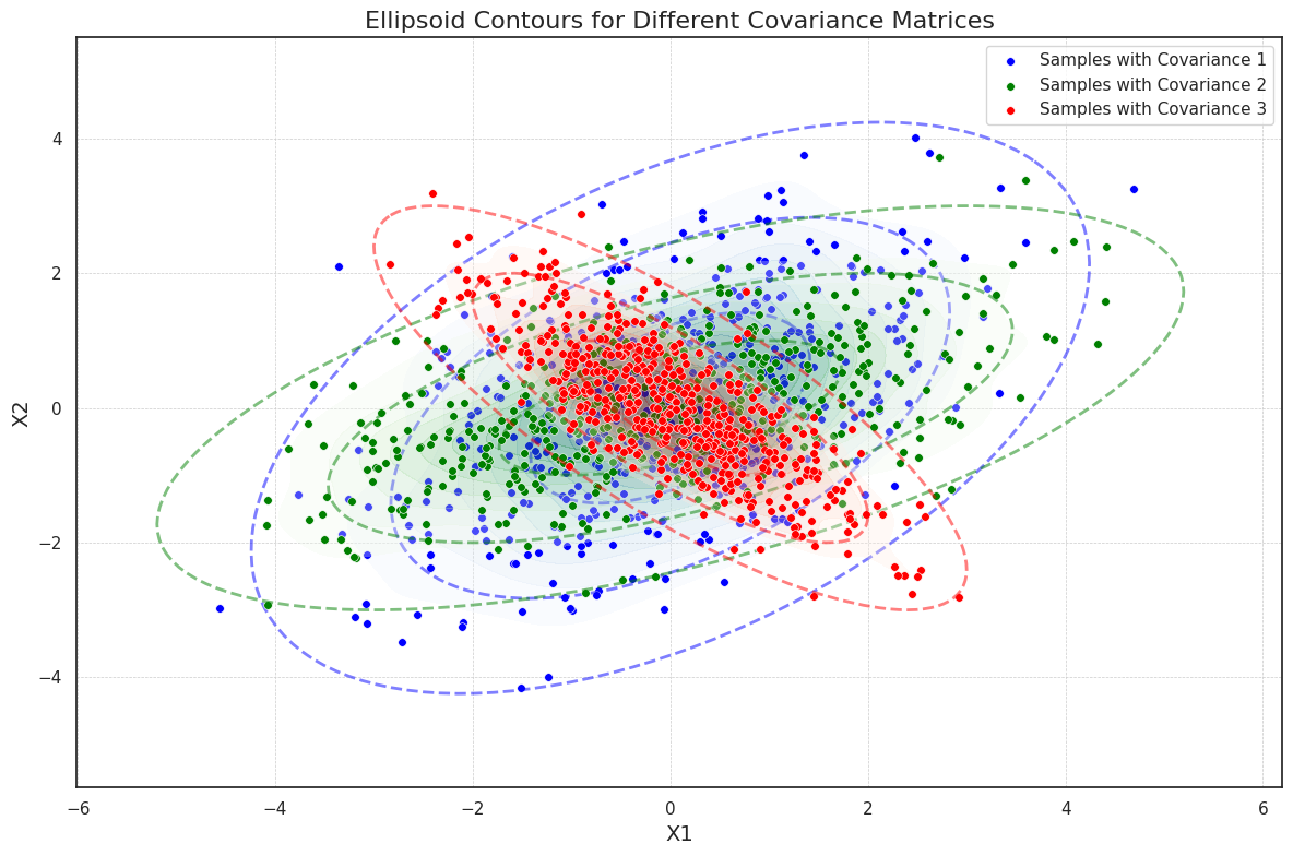
Demo for the Ellipsoid Theorem

To illustrate this, we generate samples from three different 2-dimensional Gaussian distributions, each with a unique covariance matrix. Each covariance matrix introduces a different level of correlation between the dimensions, which changes the orientation and shape of the ellipsoidal contours. We visualize these contours using concentric ellipses representing one, two, and three standard deviations from the mean. These ellipses are derived from the eigenvalues and eigenvectors of the covariance matrices, where the eigenvalues define the axis lengths, and the eigenvectors determine the rotation of each ellipse. The final plot overlays scatter plots of each Gaussian sample set to show sample density, and the ellipsoid contours at multiple standard deviations.

import numpy as np
import seaborn as sns
import matplotlib.pyplot as plt
from scipy.stats import multivariate_normal
from matplotlib.patches import Ellipse

# Set experiment parameters
mu = [0, 0]  # Mean vector
covariances = [
    [[2, 1], [1, 2]],  # Covariance matrix 1
    [[3, 1], [1, 1]],  # Covariance matrix 2
    [[1, -0.8], [-0.8, 1]]  # Covariance matrix 3
]

# Generate samples for each covariance matrix
np.random.seed(42)
samples = [np.random.multivariate_normal(mu, cov, 500) for cov in covariances]  # 500 samples per covariance matrix

# Set up plot
plt.figure(figsize=(12, 8))

# Define colormaps and colors for each covariance matrix
colormaps = ["Blues", "Greens", "Reds"]
colors = ["blue", "green", "red"]

# Plot sample distributions and ellipsoid contours
for i, (sample, cov) in enumerate(zip(samples, covariances)):
    # Density plot for samples with KDE
    sns.kdeplot(x=sample[:, 0], y=sample[:, 1], fill=True, cmap=colormaps[i], alpha=0.3, thresh=0.1)
    # Scatter plot for samples with explicit color
    sns.scatterplot(x=sample[:, 0], y=sample[:, 1], s=30, color=colors[i], label=f"Samples with Covariance {i+1}")

    # Draw ellipsoids for 1, 2, and 3 standard deviations
    eigenvalues, eigenvectors = np.linalg.eigh(cov)  # Eigenvalues and eigenvectors for covariance matrix
    angle = np.degrees(np.arctan2(*eigenvectors[:, 0][::-1]))  # Rotation angle in degrees
    for n_std in range(1, 4):  # 1, 2, 3 standard deviations
        width, height = 2 * n_std * np.sqrt(eigenvalues)  # Ellipse width and height
        ellipse = Ellipse(xy=mu, width=width, height=height, angle=angle,
                          edgecolor=colors[i], linestyle="--", linewidth=2, fill=False, alpha=0.5)
        plt.gca().add_patch(ellipse)

# Add title and axis labels
plt.title("Ellipsoid Contours for Different Covariance Matrices", fontsize=16)
plt.xlabel("X1", fontsize=14)
plt.ylabel("X2", fontsize=14)
plt.legend(loc="upper right")

# Beautify the plot
plt.grid(True, which="both", linestyle="--", linewidth=0.5)
plt.tight_layout()
plt.show()

Conclusion

In this blog, we introduced the key properties of the multivariate Gaussian distribution, including the independence of random variables, the derivation of marginal and conditional distributions, closure under linear transformations, and its geometric characteristics. These properties form the foundation of probabilistic modeling and serve as building blocks for more complex models.

As a natural extension of the multivariate Gaussian distribution, Gaussian Mixture Models (GMMs) combine multiple Gaussian components to flexibly capture multimodal characteristics in data. In the next blog, we will explore the mathematical principles behind GMMs and their applications as generative models.